 Run click the button to execute the code.
  Graph click the button to plot the data as shown.
 Band Prediction |
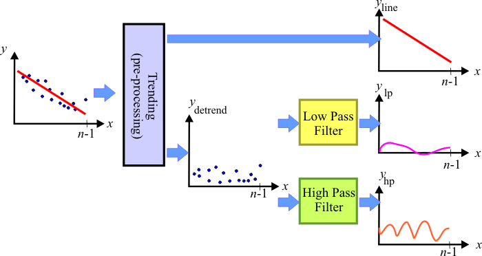
| In most series, the data follows periodic patterns that can be analyzed separately. Thus, the original series y may be divided in three (or more) new series. For instance, one typical set of new series may be: yline, ylp and yhp. The concept of band prediction is shown in the figure (note that lp stands for low pass and hp for high pass). |
| Tip |
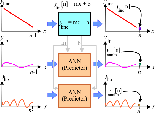
| It is possible to predict a value for each of the new series, and the total prediction value can be obtained by adding each of the predictions as shown in the figure below. |
| Tip |
A prediction problem by removing the trend of the series using band frequencies has five steps as described in the figure below.
|
| Problem 1 |
| Create a Neural Lab project called BandPred to predict the temperature in a small city in Europe using band prediction (select the Prediction option in the New Project dialog). Perform STEP 1. (a) Compute the value of m and b of the line y = mx + b that best fits the data. (b) Remove the trend from the original series to create ydetrend. |
| Solution 1 |
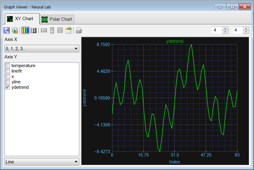
Add the RemoveTrend.lab file and write the code shown below.  Run click the button to execute the code. Run click the button to execute the code.  Graph click the button to plot the data as shown. Graph click the button to plot the data as shown. |
| BandPred\RemoveTrend.lab |
| Vector temperature; temperature.Load(); int length = temperature.GetSize(); Vector linefit = temperature.LineFit(); double m = linefit[0]; double b = linefit[1]; linefit.Save(); //_____________________ Create a line to display Vector x; x.CreateSeries(0, length-1, length); Vector yline = m*x+b; //_____________________ Remove the trend Vector ydetrend = temperature - yline; ydetrend.Save(); |
| Problem 2 |
| Plot the spectum of ydetrend. |
| Solution 1 |
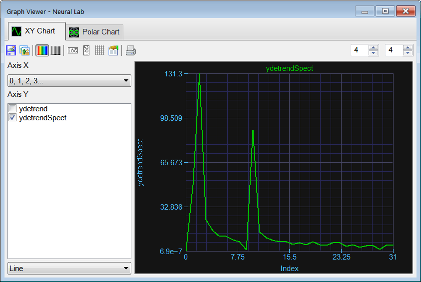
Add the Spectrum.lab file and write the code shown below. Run click the button to execute the code. Run click the button to execute the code.  Graph click the button to plot the data as shown. As it can be seen from the plot the series has two main frequency components: 0.28 radians (2.8*π/32) and 0.96 radians (9.8*π/32); Graph click the button to plot the data as shown. As it can be seen from the plot the series has two main frequency components: 0.28 radians (2.8*π/32) and 0.96 radians (9.8*π/32); |
| BandPred\Spectrum.lab |
| Vector ydetrend; ydetrend.Load(); Vector ydetrendSpect = spectrum(ydetrend); |
| Problem 3 |
| (a) Create a low pass filter with cut frequency of 0.6 radians. (b) Plot the frequency response of the filter. |
| Solution 3 |
Add the FilterResponse.lab file and write the code shown below. Run click the button to execute the code. Run click the button to execute the code. |
| BandPred\FilterResponse.lab |
| Vector impulseResponseLP; impulseResponseLP.CreateLoPassIR(5, 64, 0.6); Vector frecResponse = spectrum(impulseResponseLP); |
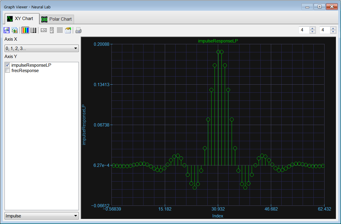
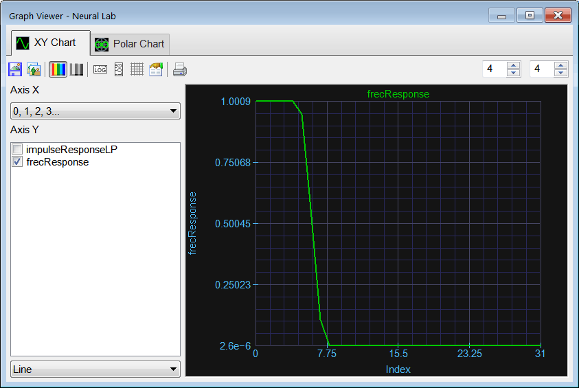
| Problem 4 |
| Continue with STEP 1. (a) Use the low pass filter to create ylp. (b) Compute yhp by subtracting ylpydetrend. |
| Solution 4 |
Add the Filtering.lab file and write the code shown below. Run click the button to execute the code. Run click the button to execute the code. |
| BandPred\Filtering.lab |
| Vector impulseResponseLP; impulseResponseLP.CreateLoPassIR(5, 64, 0.6); //_______________________________ Vector ydetrend; ydetrend.Load(); Vector ylp = ShortConvolution(ydetrend, impulseResponseLP); Vector yhp = ydetrend - ylp; ylp.Save(); yhp.Save(); |
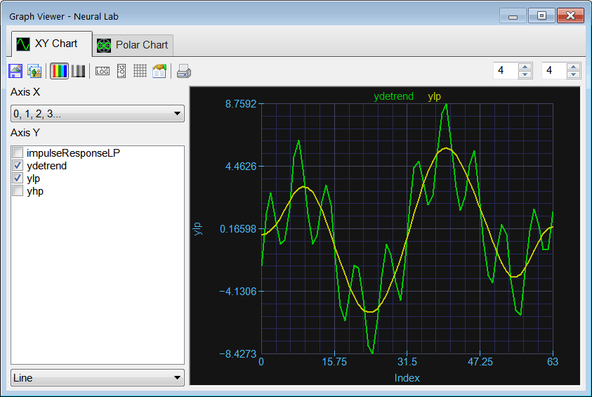
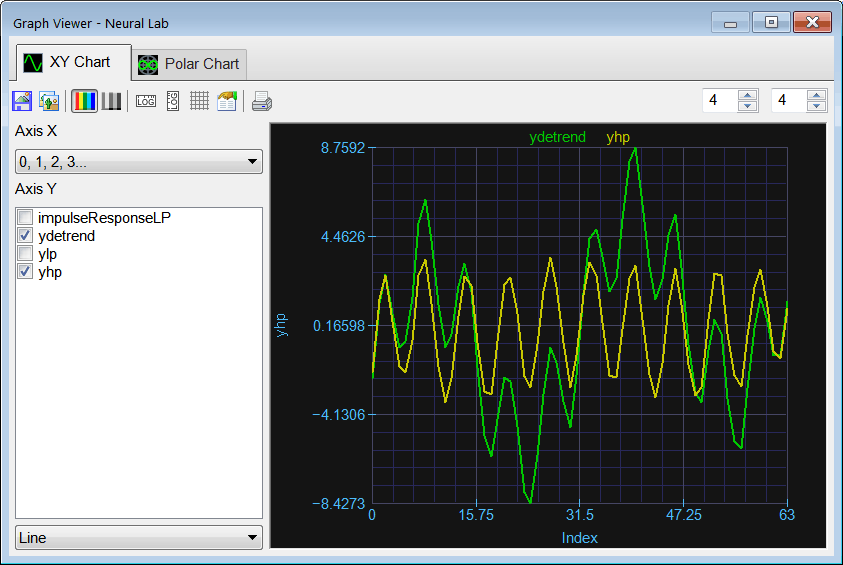
| Problem 5 |
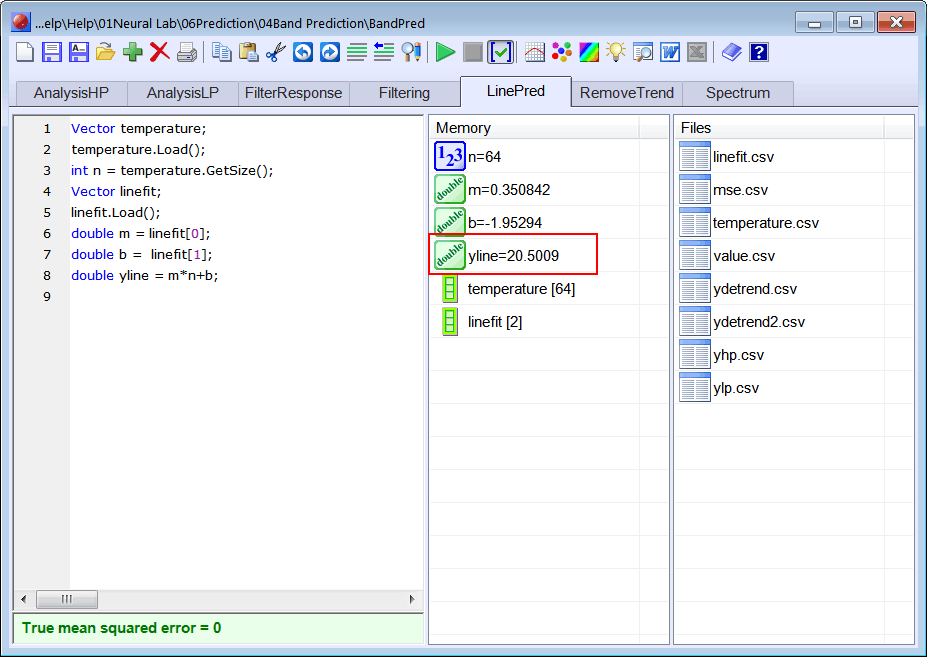
| Perform STEP 2. Estimate the line prediction using the equation of the line. That is estimate yline[64]. |
| Solution 5 |
Add the LinePred.lab file and write the code shown below. Run click the button to execute the code. Run click the button to execute the code. |
| BandPred\LinePred.lab |
| Vector temperature; temperature.Load(); int n = temperature.GetSize(); Vector linefit; linefit.Load(); double m = linefit[0]; double b = linefit[1]; double yline = m*n+b; |
| Problem 6 |
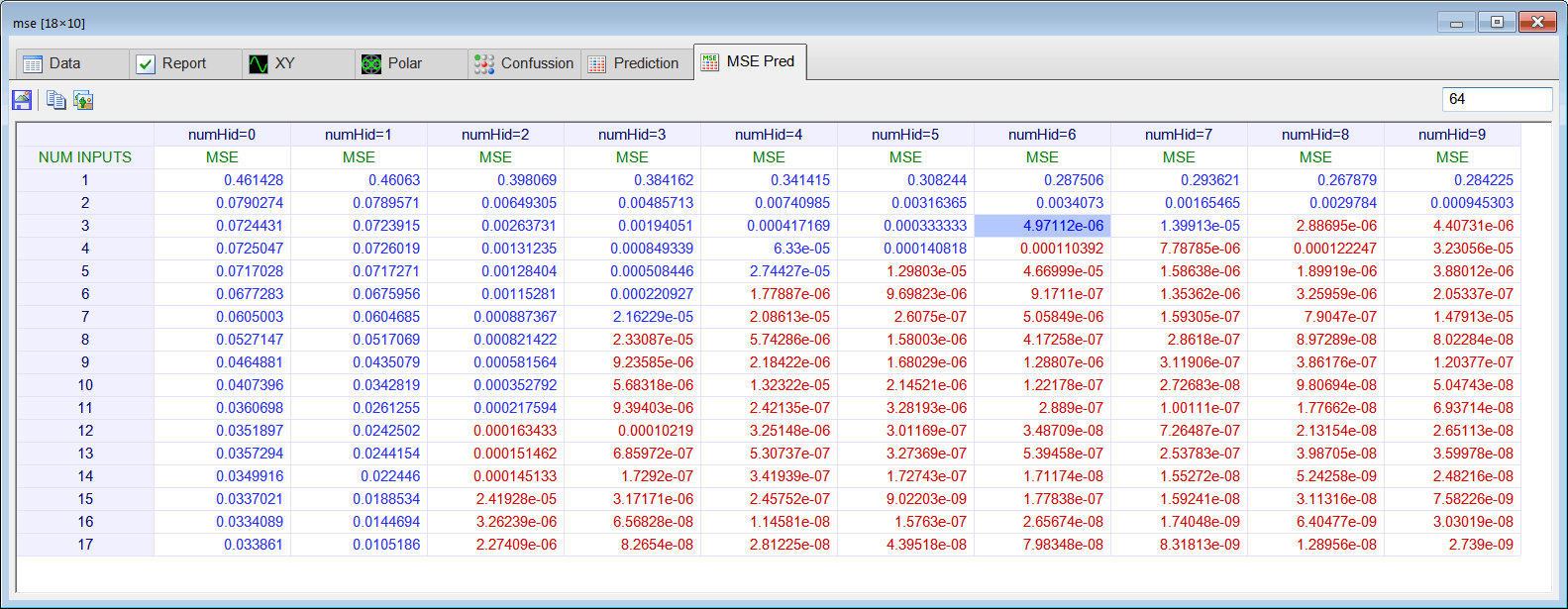
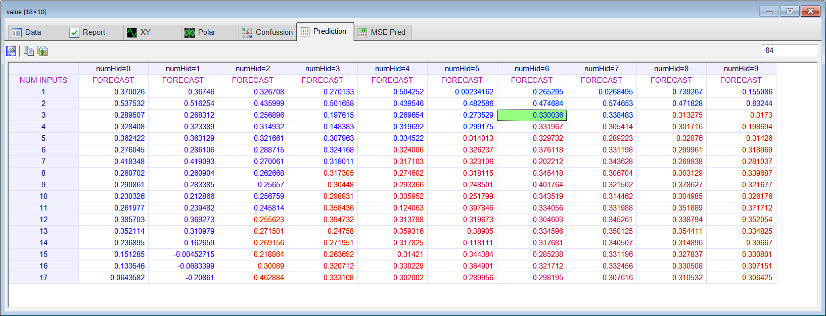
| Perform STEP 3. Estimate yannlp[64] using prediction analysis by writing the PredAnalysisLP.lab file. |
| Problem 7 |
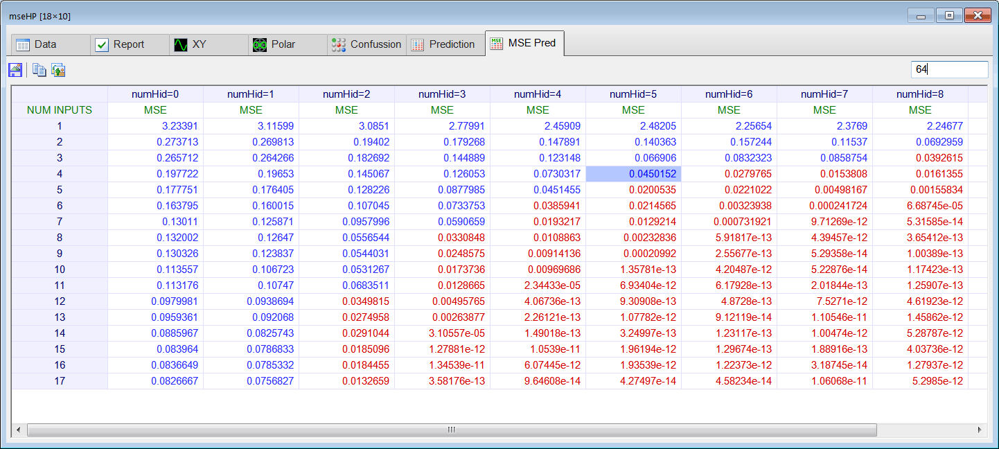
| Perform STEP 4. Estimate yannhp[64] using prediction analysis by writing the PredAnalysisHP.lab file. |
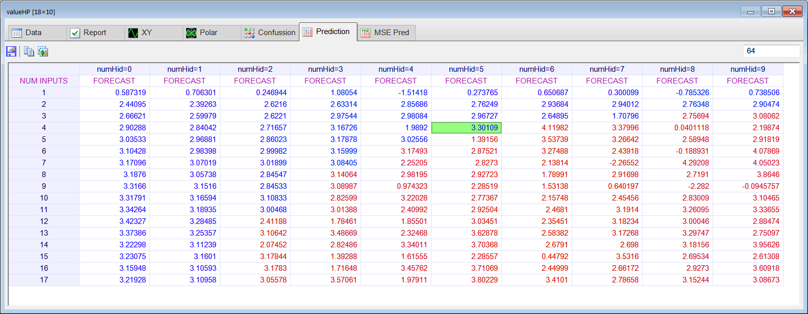
| Problem 8 |
| Perform STEP 5. Combine the line prediction with the ANN prediction to estimate y[64]. |
| Series Length | Actual Value | yline[64] | yannlp[64] | yannhp[64] | Estimate of y[64] |
| 64 | y[64]=23.75 |
| Problem 9 |
| Create the Validation.lab file to perform the prediction validation. (a) By removing values at the end of the series ydetrend complete the table below with the predicted value using an ANN. (b) Compute the mse between the actual and the predicted values using the 10 values in the table. |
| Series Length | Actual Value | yline | yannlp | yannhp | Estimate of y |
| 63 | y[63]=21.46 | ||||
| 62 | y[62]=18.52 | ||||
| 61 | y[61]=18.17 | ||||
| 60 | y[60]=19.46 | ||||
| 59 | y[59]=20.27 | ||||
| 58 | y[58]=18.40 | ||||
| 57 | y[57]=15.14 | ||||
| 56 | y[56]=11.91 | ||||
| 55 | y[55]=11.91 | ||||
| 54 | y[54]=13.64 |